Digging Into AI Forecasts: Are They Physically Sound?
Over the past few years, deep learning (DL) based weather models have made significant progress in short- and medium-range forecasting. Models like FourCastNet, GraphCast, and Pangu-Weather now rival or even outperform traditional numerical weather prediction (NWP) models in terms of raw skill scores like RMSE or ACC.
However, while these scores tell us what the model predicts, they reveal little about how the model arrives at its predictions. Does it capture physical relationships like energy conservation, hydrostatic balance, or the influence of temperature gradients on cyclone intensification? Or is it simply exploiting statistical shortcuts hidden in the data?
This is where physical interpretability becomes crucial. It’s not just about opening the black box, it’s about evaluating whether the model’s internal logic aligns with established physical principles. For high-stakes forecasting, like hurricanes, heatwaves, or flooding, this kind of trust and understanding is essential.
In this article, we explore one method that has been proposed for establishing physical interpretability: comparing sensitivity fields derived from AI models and traditional adjoint models. This article is based on the paper by Baño-Medina et al.
Adjoint Models: A Tool from NWP to Probe Sensitivities
In traditional NWP, adjoint models are mathematical tools used for sensitivity analysis. They efficiently compute gradients of forecast outputs with respect to input perturbations, providing insights into how changes in inputs like initial conditions, boundary conditions, or model parameters influence forecast behavior.
The process begins by defining a scalar objective function, typically denoted as $J$, that quantifies some aspect of the forecast output—such as the mean squared error, or the total precipitation over a region and time period. We also define a control state $a_c$, representing the unperturbed input.
Tangent linear models are used as a foundation for adjoint models, leveraging the chain rule for derivatives. The tangent linear model is expressed as linear perturbations of input and output using first-order Taylor approximations.
Adjoint models are based on tangent linear models, which approximate how small perturbations in the input state lead to linearised changes in the output, using a first-order Taylor expansion. This provides the foundation for applying the chain rule of derivatives.
Suppose we introduce a small perturbation $\delta a$ around the control solution. Since $J$ depends on the model output $b$, not directly on $a$, we begin by expressing how small changes in $b$ affect $J$, using:
\[\Delta J = \sum_k \frac{\partial J}{\partial b_k}\delta b_k\]This tells us how the objective function changes in response to small output variations. But because the output $b$ itself is a function of the input $a$, we can similarly write:
\[\Delta b_j = \sum_k \frac{\partial b_j}{\partial a_k}\delta a_k\]By applying the chain rule, we then obtain the key result:
\[\frac{\partial J}{\partial a_j}=\sum_k \frac{\partial b_k}{\partial a_j} \frac{\partial J}{\partial b_k}\]This expression gives us the sensitivity of the forecast metric $J$ to changes in each input variable $a_j$. The adjoint model computes this gradient efficiently, even for very high-dimensional systems, by propagating sensitivity information backward through the model, from outputs to inputs.
Crucially, the impact of a perturbation depends not just on its magnitude, but on where and how it is introduced. A small change in temperature at a dynamically sensitive atmospheric layer may strongly affect cyclone development, whereas a similar perturbation in a less influential region might have little to no impact. Adjoint models help identify these key sensitivities, making them indispensable for data assimilation, error tracking, and, increasingly, model analysis.
Automatic Differentiation
In DL models, particularly those built with frameworks like PyTorch or JAX—we can compute sensitivities using automatic differentiation, a technique for efficiently computing exact derivatives of functions expressed as compositions of elementary operations.
PyTorch’s autograd engine implements reverse-mode automatic differentiation, which is especially efficient for functions with many inputs and a single scalar output, such as the loss functions used in deep learning and weather forecasting.
Suppose we have a scalar-valued function $y=f(\vec{x})$, where $\vec{x}\in\mathbb{R}^n$. Automatic differentiation decomposes $f$ into a computational graph of basic operations (e.g., additions, multiplications, activation functions). The gradient $\nabla f$ is then computed using the chain rule in two passes:
Forward Pass: Break \(f\) into a sequence of intermediate computations \(v_i\):
\[\begin{aligned} v_1 &= x_1, \\ v_2 &= x_2, \\ &\vdots \\ v_k &= g_k(\text{inputs of } g_k) \end{aligned}\]Here each \(g_k\) is a basic operation (e.g., addition, multiplication, \(\sin\), \(\exp\)), and its inputs are the variables it directly depends on (its parents in the computation graph).
Backward Pass: Compute gradients via the chain rule, propagating derivatives backward from \(y\):
\[\frac{\partial y}{\partial v_i}= \sum_{v_j \in \text{dependents of } v_i}\frac{\partial y}{\partial v_j} \cdot \frac{\partial v_j}{\partial v_i}\]Where:
- \(\frac{\partial y}{\partial v_j}\) is the gradient flowing into \(v_j\) from its dependents (children in the graph)
- \(\frac{\partial v_j}{\partial v_i}\) is the local derivative of \(v_j\) w.r.t. \(v_i\)
This backward gradient propagation in autograd is conceptually identical to what adjoint models do in numerical weather prediction. Both systems apply the chain rule in reverse, tracing how a scalar-valued outcome (like loss or cost) depends on high-dimensional inputs.
A key difference is that in NWP adjoint models are derived from differentiating physical equations (e.g., discretized PDEs governing fluid dynamics), often implemented manually or semi-automatically, while in deep learning, automatic differentiation works on computational graphs, enabling general-purpose, automatic gradient computation for any differentiable function composed of elementary operations.
Despite this difference in implementation, both frameworks provide gradients that quantify how a scalar output depends on a complex chain of intermediate variables, making them powerful tools for sensitivity analysis and model interpretability.
Physical Interpretability
Both NWP models and AI-based weather models can produce sensitivity fields, maps showing how perturbations in the initial conditions influence a forecast metric. In NWP, these fields are derived using adjoint models; in AI models, we compute them via automatic differentiation. Comparing the two provides a direct way to assess whether the AI model captures meaningful physical relationships.
This approach is the focus of the recent paper “Are AI weather models learning atmospheric physics? A sensitivity analysis of cyclone Xynthia” by Baño-Medina et al, the authors examine FourCastNetv2, an DL weather model, and compare its sensitivity maps to those from a traditional adjoint model, using cyclone Xynthia (a major European windstorm from 2010) as a case study.
In both models, the objective function is the kinetic energy (KE) at 36-hour lead time, computed over the Bay of Biscay. The KE is defined as the spatial average of squared wind components:
\[KE=0.5 \sum_{i}\frac{u_i^2+v_i^2}{N}\]where $u_i$ and $v_i$ are the zonal and meridional wind components at grid point $i$, and $N$ is the number of grid points in the region.
In FourCastNetv2, the gradient of KE with respect to the initial conditions is computed using PyTorch’s autograd engine, applying the chain rule through backpropagation. In the NWP model, the same gradient is obtained via the adjoint of a physics-based numerical model.
The figure below shows side-by-side comparisons of sensitivity fields from the adjoint model (a, b, c) and the AI model (d, e, f). Warm colors indicate regions where small increases in the initial values lead to higher KE at the forecast time, while cold colors indicate regions where decreases have the same effect.
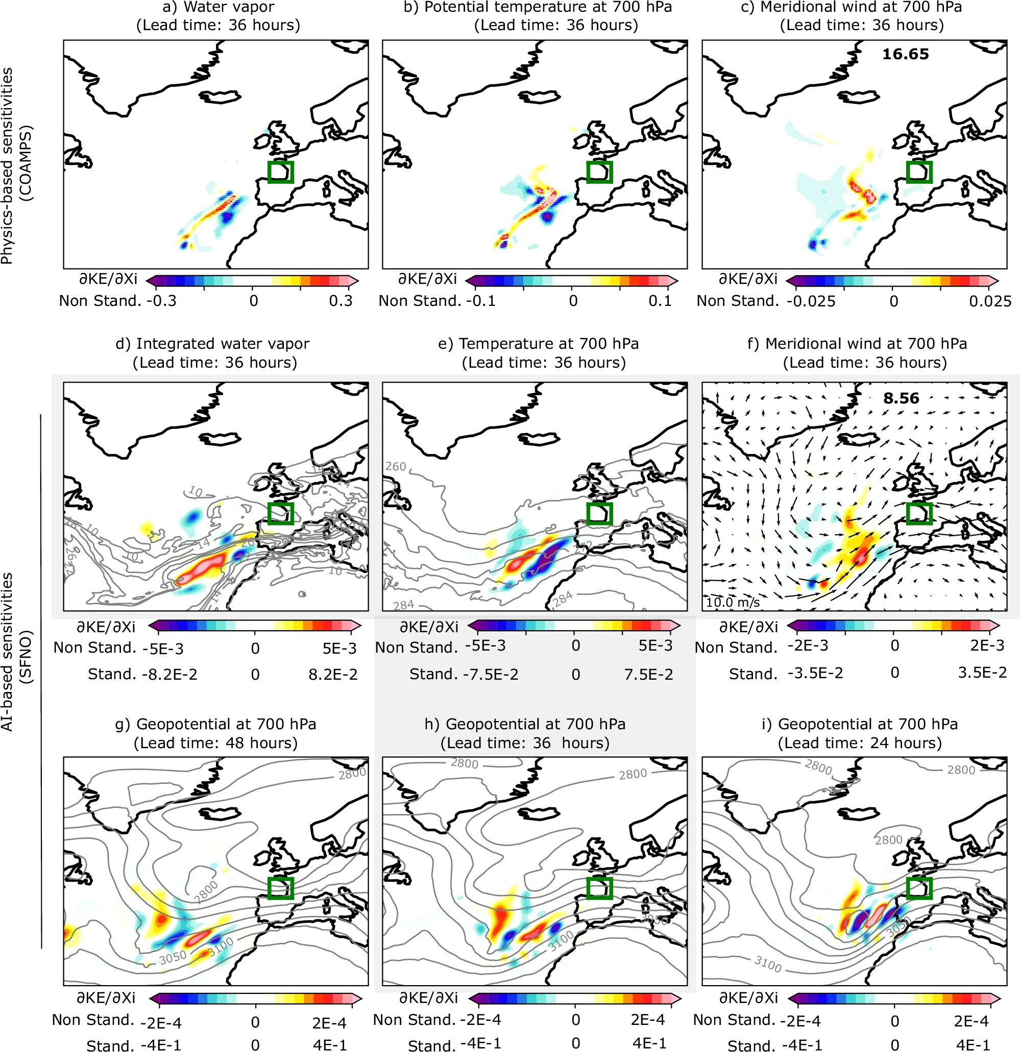
The comparison reveals striking agreement between the two methods. For example, the meridional wind sensitivity shows a characteristic S-shaped structure west of Portugal, which appears clearly in both the adjoint (c) and the AI model (f). This suggests that the AI model has learned a physically meaningful mechanism for cyclone intensification.
The next figure shows a vertical cross-section of sensitivity to relative humidity in the AI model, compared to specific humidity sensitivities from the physics-based model along the same northwest–southeast transect.
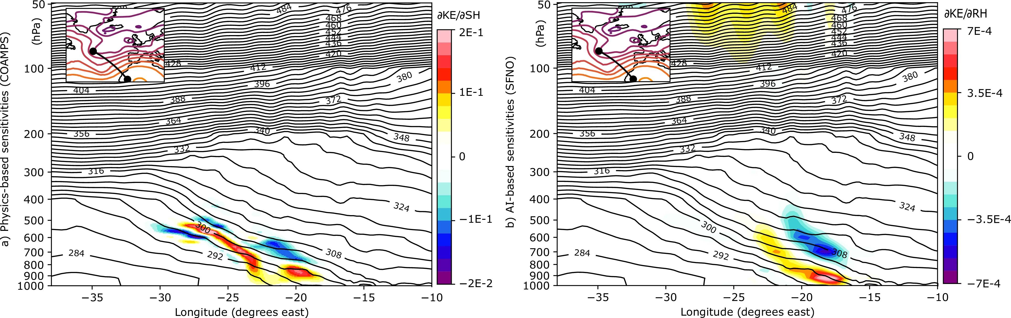
Overall, the vertical structure of the sensitivity fields aligns well between the two models. However, the AI model exhibits a positive sensitivity at upper atmospheric levels not present in the adjoint output. Since there is no known physical mechanism linking these upper-level features to low-level KE, this may indicate a spurious or non-physical correlation learned by the neural network.
Identifying such artifacts is essential. They highlight areas where the model might be overfitting or relying on statistically useful but physically implausible patterns, issues that must be addressed if AI weather models are to gain the same level of trust as traditional models.
Looking Ahead
Comparing sensitivity fields between AI and adjoint-based NWP models is a powerful method for evaluating physical interpretability. It bridges the gap between performance and understanding, offering a concrete way to test whether AI models are truly learning atmospheric physics, or merely mimicking it.
In a future article, we’ll continue along this line of inquiry by analysing the sensitivity fields of Pangu-Weather, another state-of-the-art AI model for global weather forecasting.