Understanding Graph Neural Networks
In this article, we’ll explore Graph Neural Networks (GNNs): what they are, how they work, and why they’re useful. We’ll walk through a practical example using a well-known graph-based dataset to solve a node classification problem with a GNN. All code used in this tutorial is available on GitHub.
What is a Graph?
At its core, a graph is a mathematical structure used to represent relationships between entities. It consists of:
- Nodes: the entities themselves
- Edges: the relationships or connections between nodes
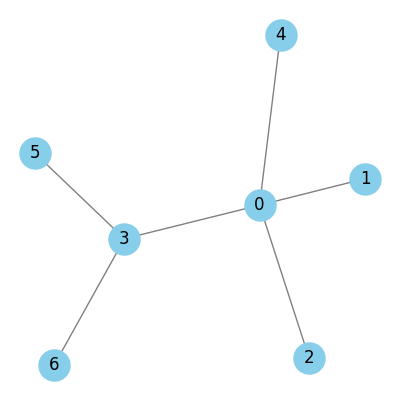
Below is a simple example:
Graphs can be undirected or directed. In directed graphs, the edges are associated with a given direction, and we distinguish the connected nodes as source and target. In many datasets, additional information is associated with nodes and edges. This is typically represented as a feature vector (a fixed-length list of numbers). For example, node attributes might represent properties like a paper’s topic in a citation network, or edge attributes could capture things like the strength or type of relationship.
In many real-world graph datasets, some of these attributes may be missing. A typical setup includes a liste of nodes, a set of node features (attribute vectors), a list of edges, and optionally edge attributes. It’s important to distinguish between the structure or connectivity of the graph, given by the edges, and the attributes of the nodes and edges.
The Cora Dataset
The Cora dataset is a citation network commonly used in graph learning benchmarks. It contains 2,708 scientific papers, each categorized into one of seven machine learning topics: Case-Based Reasoning, Genetic Algorithms, Neural Networks, Probabilistic Methods, Reinforcement Learning, Rule Learning, and Theory.
Each node represents a paper. If paper A cites paper B, there is a directed edge from A (source) to B (target). These connections form the structure of the graph.
To represent the graph’s structure, we use the edge index, a tensor of shape (2, M) where M is the number of edges. The first row contains the source nodes of each edge, and the second row contains the corresponding target nodes. For example, if the first entry in the edge index is [633, 0], it means there is a citation from node 633 to node 0. In Cora, there are 10,556 edges in total.
We also have a label vector of length 2,708. It tells us the ground truth class of each paper. These labels are not passed as input to the GNN. Instead, they’re used during training to supervise the model.
The machine learning task we’re tackling is node classification: predicting the topic of each paper based on its content and its citation links.
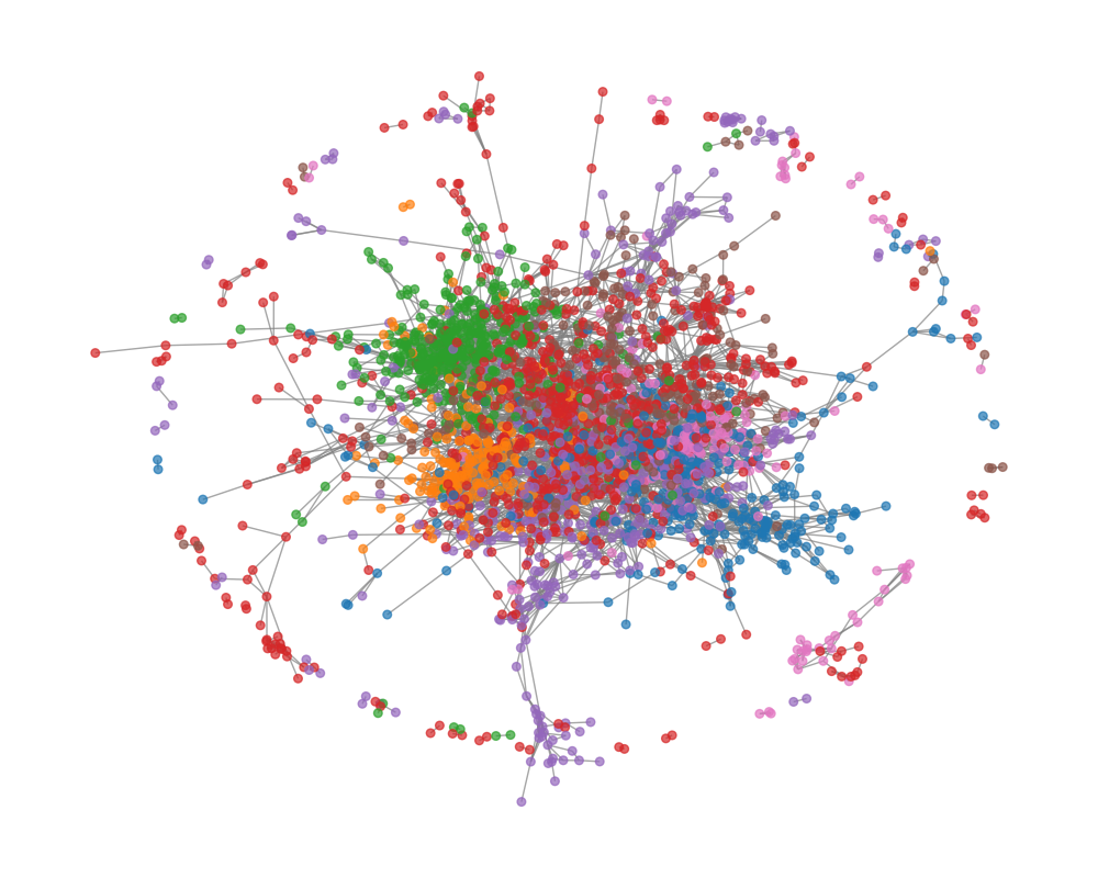
Below is a visualisation of the Cora graph. Each node is color-coded according to its class. As you can see, there’s a densely connected core, representing a tightly interlinked group of papers, and also more loosely connected clusters around the periphery.
Using a Simple Neural Network (Without the Graph)
Before diving into graph neural networks, it’s useful to establish a baseline using a standard neural network that does not use the graph structure. For this, we implement a Multi-Layer Perceptron (MLP), which treats each paper independently based only on its feature vector.
This setup allows us to evaluate how much predictive power comes from the node features alone, without considering the citation links between papers.
In this approach, we:
- use only the node feature matrix of shape (2708, 1433) as input.
- ignore the edge index and any information about how papers cite each other.
- train the MLP to predict the class of each paper.
import torch
import torch.nn.functional as F
from torch_geometric.datasets import Planetoid

# Load Cora dataset
dataset = Planetoid(root='data/Cora', name='Cora')
data = dataset[0]

# Define MLP
class MLP(torch.nn.Module):
    def __init__(self, in_channels, hidden_channels, out_channels):
        super().__init__()
        self.fc1 = torch.nn.Linear(in_channels, hidden_channels)
        self.fc2 = torch.nn.Linear(hidden_channels, out_channels)

    def forward(self, x):
        x = self.fc1(x)
        x = F.relu(x)
        x = self.fc2(x)
        return F.log_softmax(x, dim=1)

model = MLP(dataset.num_node_features, 64, dataset.num_classes)

# Train
optimiser = torch.optim.Adam(model.parameters(), lr=0.01, weight_decay=5e-4)

model.train()
for epoch in range(200):
    optimiser.zero_grad()
    out = model(data.x)
    loss = F.nll_loss(out[data.train_mask], data.y[data.train_mask])
    loss.backward()
    optimiser.step()

# Evaluate
model.eval()
pred = model(data.x).argmax(dim=1)
correct = pred[data.test_mask] == data.y[data.test_mask]
acc = int(correct.sum()) / int(data.test_mask.sum())
The last time this was run, the accuracy was about 56.6%. Not the most inspiring figure. In the next section, we’ll see if we can improve the model’s accuracy by leveraging the graph structure of the dataset.
Using a Graph Neural Network
Now we implement a Graph Neural Network (GNN) to solve the same classification task. To ensure a fair comparison with the MLP, we’ll keep the architecture similar: two layers, with a ReLU activation in between, followed by softmax for classification. The key difference is that instead of standard linear layers, we’ll use graph layers.
There are many types of graph layers, depending on how information is propagated between nodes. In this tutorial, we’ll use the Graph Convolutional Network (GCN) layer introduced by Kipf & Welling. PyTorch Geometric provides a built-in implementation (torch_geometric.nn.GCNConv), but we’ll implement it from scratch to better understand the underlying mechanics. If you’re looking for speed or scalability, you should use the built-in version.
Inputs and Outputs of a GNN Layer
Before going into the layer details, it’s important to understand the input/output interface of a graph layer.
In PyTorch Geometric, a graph is typically represented by two components:
x: the node feature matrix of shape(N, F_in), whereNis the number of nodes (2708 for Cora), andF_inis the input feature dimension (1433).edge_index: a tensor of shape(2, E), where each column is a pair of node indices(i, j)indicating a directed edge from nodeito nodej(10556 edges in Cora).
The output of a GNN layer is a new node feature matrix of shape (N, F_out). The edge index stays the same: it defines the structure of the graph and should not be modified. Changing it would mean altering the actual graph connectivity, which is a separate operation.
Key Steps in the GCN Layer
A Graph Convolutional Network (GCN) layer typically consists of three main steps:
- Linear transformation
- Degree normalization
- Message passing
Let’s walk through each of them in detail.
1. Linear Layer
The linear transformation is applied to the node feature matrix without using any graph structure. For the Cora dataset, this means applying a linear layer to the (2708 × 1433) input matrix. The output dimension of the layer is user-defined—in our case, we choose a hidden dimension of 64.
This operation is simply:
\[H'=H^{(l)}W^{(l)}\]Where $H^{(l)}$ is the input feature matrix of the $l$ th layer, $W^{(l)}$ is the learnable weight matrix of the $l$ th layer, and $H’$ is the resulting feature matrix. We refer to the result as the embedded node matrix, and each row in this matrix as an embedded node. At this stage, we haven’t yet incorporated the graph structure. That comes next.
2. Degree Normalisation
Before performing message passing, we compute degree normalization factors, which help scale messages and prevent numerical instability. Although not strictly required, this step is essential for the stability and performance of GCNs.
To understand normalisation, we first introduce the concept of an adjacency matrix $A$, which is one way to represent graph structure. In an adjacency matrix, rows correspond to source nodes, columns correspond to target nodes, and a value of 1 is populated when an edge exists between the nodes, 0 otherwise.
Using a small toy graph (see Fig. 1), its adjacency matrix is (blue means 1, white means 0:
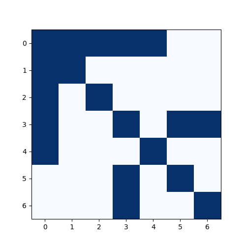
Importantly, here we have added self-loops, i.e., we consider every node to be connected to itself. This results in 1’s along the diagonal. While adjacency matrices by default exclude self-connections, adding them is crucial in GCNs because it allows each node to retain its own features during aggregation (see message passing).
We then compute the degree matrix $D$, which is a diagonal matrix where each diagonal entry $D_{ii}$ is the number of neighbors (including itself) that node $i$ has:
\[D_{ii}=\sum_j A_{ij}\]Finally, we apply symmetric normalisation to the adjacency matrix, defined as:
\[\tilde{A}=D^{-\frac{1}{2}}AD^{-\frac{1}{2}}\]While this looks more complicated, $\tilde{A}$ retains the same structure as the original adjacency matrix. However, instead of binary values (1s and 0s), each entry now holds a weight that reflects the connectivity between nodes, scaled by their degrees. This weighting is important because it preserves the graph structure while incorporating degree information.
We won’t apply the normalisation matrix just yet, it will come into play during the message passing step. By incorporating it there, we ensure that feature aggregation does not overly favor high-degree nodes and that the scale remains consistent across the graph.
3. Message Passing
Message passing is the core mechanism that gives Graph Neural Networks their power. It allows each node to incorporate information from its neighbors, capturing the structure of the graph and enabling more context-aware predictions.
While there are many variations of message passing across different GNN architectures, the core idea is consistent: nodes exchange and aggregate information via the edges that connect them.
Message passing can conceptually be applied nodes and edges, or even combinations of them. However, the applicability depends on what attributes are present. For example, if the graph lacks edge features, we can’t perform message passing on edges—but we can still pass messages via edges between nodes.
In the GCN model, we perform message passing on nodes only. Let’s revisit node 0 from our toy graph (Fig. 1). Node 0 is connected to nodes 1, 2, 3, and 4. In the message passing step, node 0 will aggregate the features of itself (thanks to the self-loops), and nodes 1, 2, 3, and 4 (its immediate neighbors).
Also in the GCN model, aggregation simply means summing the feature vectors of neighboring nodes. However, since we are incorporating normalisation, this becomes a weighted sum. Specifically, before summing, each neighbor’s feature vector is multiplied by the corresponding weight from the normalisation matrix, i.e. the entry $\tilde{A}_{ij}$, where node $j$ is directed to node $i$.
And that’s it. As stated previously, message passing is fairly simple, but time and time again, it has been proven to be an effective method for encoding the graph’s connectivity.
There are a few more things to note about message passing. Firstly, GCN layers only aggregate information from immediate neighbors (1-hop connections). This means that long-range dependencies are not captured in a single layer. To capture longer-range relationships, we stack multiple GCN layers. For instance, if nodes are three hops apart, it will take three GCN layers to propagate information between them. Also, Each layer typically has its own set of weights (i.e., different linear transformations). So a 2-layer GCN will have two different sets of parameters, one per layer.
Each additional layer performs another full round of linear transformation → normalisation → message passing. This layered structure allows the model to build up increasingly abstract representations of the graph structure and node content.
Finally, the message passing operation described above can be expressed compactly using matrix multiplication. In the original GCN paper, the graph layer is written as:
\[H^{(l+1)}=\sigma(D^{-\frac{1}{2}}AD^{-\frac{1}{2}}H^{(l)}W^{(l)})\]Here, we can see that the normalisation matrix is being multiplied by linear activation matrix, and this constitutes the whole message passsing. Of course, an activation function wraps the entire operation.
The reason why matrix multiplication performs the desired message passing is because the normalisation matrix $\tilde{A}$ (via the adjacency matrix) encodes the connected nodes for aggregation. Each row $i$ in the normalisation matrix corresponds to node $i$. Non-zero entries in that row correspond to nodes connected to $i$ (including itself, since we added self-loops). Therefore, matrix multiplication sums up the features of all neighboring nodes (weighted appropriately), and excludes non-neighbors due to the zero entries in $\tilde{A}$.
This equivalence allows us to avoid explicit for-loops over neighbors during implementation, making the computation more efficient. It’s still slower than the highly optimised implementation in PyTorch Geometric’s, but it will save us a lot of time (I tried all options).
class GNNLayer(torch.nn.Module):

    def __init__(self, in_channels, out_channels):
        super().__init__()
        self.in_channels = in_channels
        self.out_channels = out_channels

        self.linear = torch.nn.Linear(in_channels, out_channels)

    def forward(self, x, edge_index, num_nodes):
        # Apply linear activations
        x = self.linear(x)

        # Construct adjacency matrix
        adj_dense = torch.zeros((num_nodes, num_nodes))
        adj_dense[edge_index[0], edge_index[1]] = 1
        adj_dense += torch.eye(num_nodes) # add self loops

        # Calculate degree normalisations
        d = adj_dense.sum(dim=1)
        d.pow_(-0.5)
        D = torch.diag(d)

        # Message passing
        return D @ adj_dense @ D @ x


class GNN(torch.nn.Module):
    def __init__(self, in_channels, hidden_channels, out_channels):
        super().__init__()
        self.gnn1 = GNNLayer(in_channels, hidden_channels)
        self.gnn2 = GNNLayer(hidden_channels, out_channels)

    def forward(self, data):
        x, edge_index, num_nodes = data.x, data.edge_index, data.num_nodes

        x = self.gnn1(x, edge_index, num_nodes)
        x = F.relu(x)
        x = self.gnn2(x, edge_index, num_nodes)
        return F.log_softmax(x, dim=1)

model = GNN(dataset.num_node_features, 64, dataset.num_classes)
optimizer = torch.optim.Adam(model.parameters(), lr=0.01, weight_decay=5e-4)

model.train()
for epoch in range(200):
    optimizer.zero_grad()
    out = model(data)
    loss = F.nll_loss(out[data.train_mask], data.y[data.train_mask])
    loss.backward()
    optimizer.step()

model.eval()
pred = model(data).argmax(dim=1)
correct = pred[data.test_mask] == data.y[data.test_mask]
acc = int(correct.sum()) / int(data.test_mask.sum()) # About 81%
After training this GCN-based model on the Cora dataset, we observe a test accuracy of 81%, which is a significant improvement over the baseline MLP (56.6%).
This demonstrates the strength of GNNs: by leveraging the graph structure, the model can aggregate useful contextual information and make more accurate predictions. In a future post, we’ll explore how GNNs are used in weather forecasting, including models like GraphCast.