Aurora: Microsoft’s Foundational Data-Driven Weather Model
Initially submitted to arXiv in May 2024, Aurora is Microsoft’s open-source foundation model for weather and climate prediction. Published in Nature in May 2025, it’s now freely available on GitHub, including both the code and the trained weights. Microsoft positions Aurora not just as another weather forecasting tool, but as a general foundation model for the atmosphere—capable of integrating diverse datasets and supporting a wide range of applications.
In this post, we’ll dive into how Aurora works under the hood and explore what makes it different from previous AI models for weather prediction.
Datasets
A major point that differentiates Aurora from previous models is its various training datasets. Most deep learning weather models in recent years have been trained primarily on ERA5, the widely used reanalysis dataset produced by ECMWF. However, for its pre-trained backbone, Aurora combines ERA5 with nine additional datasets, spanning different spatiotemporal resolutions, sets of variables, and numbers of pressure levels. It goes even further for its downstream fine-tuning, where depending on the task, the model is fine-tuned on an additional one or two datasets. This is a major break from previous models such as FourCastNet and GraphCast, that were only trained on a single dataset, ERA5.
This allows the model to learn from diverse sources of information, ranging from global climate reanalyses to higher-resolution simulations and observational datasets. Such heterogeneity is central to Aurora’s design, because it allows the model to remain flexible across tasks that differ in scale, variable coverage, or domain.
At the same time, heterogeneity poses a challenge for the model’s architecture. In other models like GraphCast or FourCastNet, the number of input variables does not change during training, whereas in Aurora’s case it might. This means the model needs to take this into account from an architectural perspective as well as a data infrastructure one.
Architecture
Aurora’s architecture follows the classic encoder-processor-decoder pattern.
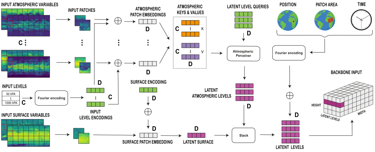
Aurora represents all variables as 2D images on a latitude–longitude grid. For each variable, we take two snapshots: the current state (t) and the previous state (t−1). Stacking these gives a small time dimension (T = 2). The model treats atmospheric and surface variables separately.
For atmospheric variables: if there are $V_A$ variables across $C$ pressure levels, the tensor looks like V_A × C × T × H × W.
For surface variables: if there are $V_S$ variables, the tensor looks like V_S × T × H × W.
Aurora also uses three “static” variables that never change with time:
- Surface geopotential (Z), which encodes topography
- Land–sea mask (LST)
- Soil-type mask (LSM)
Like in Vision Transformers, the H×W grids are split into P×P patches. Each patch is mapped to a vector of dimension D.
- For atmospheric variables:
C × V_A × T × P × P → C × D. - For surface variables:
VS × T × P × P → 1 × D.
Because datasets differ in what variables they provide, each variable $v$ has its own projection weights $W_v$, meaning that each variable type is passed through its own multi-layer perceptron with variable-specific weights.
To account for vertical structure, embeddings are tagged with level encodings. Pressure levels are represented either by a sinusoidal encoding of the pressure value (e.g. 150 hPa) for atmospheric data or by learned vectors of size $D$ for surface data.
Since different datasets have different numbers of atmospheric pressure levels, these embeddings are then aggregated through a Perceiver module, in which latent query vectors attend to the encoded pressure levels. In particular, the latent query vector has a size of $C_L=3$ such that the latent representation is $C_L \times D$. This essentially maps a variable number of pressure levels, C (depending on the dataset), to a fixed set, $C_L$.
In parallel, the surface embedding goes through a residual MLP. The outputs are concatenated to form a $(C_L + 1) \times D$ representation of the full weather state at each patch.
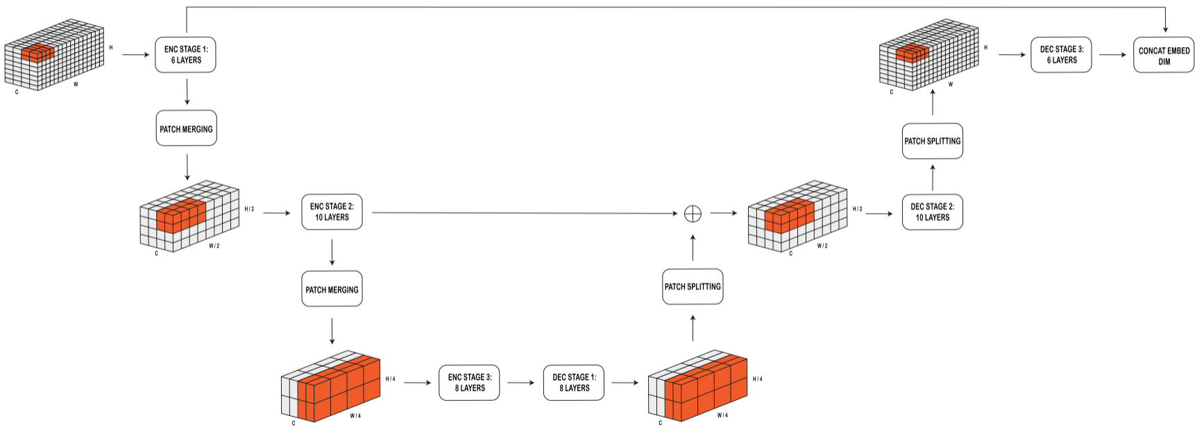
The latent 3D grid produced by the encoder can be seen as a mesh on which the simulation takes place. The backbone then acts as the neural simulator. Aurora uses the Transformer as the baseline architecture.
Aurora uses a 3D Swin Transformer U-Net backbone. It has an encoder and a decoder (these are separate to the encoder/decoder of the entire Aurora model), each made of three stages:
- After each encoder stage, the spatial resolution is halved.
- After each decoder stage, the resolution is doubled and combined with the matching encoder outputs.
Each layer applies 3D Swin Transformer blocks, where self-attention is restricted to local regions (called windows). To allow information to spread further, windows are shifted by half their size along each axis at every other layer. Because the Earth is spherical, the windows wrap around longitudinally, ensuring continuity across the globe. This design mimics the local computations of numerical solvers, but avoids the quadratic cost of vanilla Transformers.
The res-post-norm stabilization from Swin v2 is applied but the standard dot-product attention from v1 (rather than cosine attention from v2) is kept. Unlike some transformer architectures that rely on positional biases, Aurora encodes positional information entirely in its input embeddings, which enables it to operate flexibly across multiple resolutions.
The decoder takes the standardised latent simulation and maps it back to images on the latitude–longitude grid. Its structure mirrors the encoder.
The three latent atmospheric pressure levels are expanded back into the original $C$ pressure levels using a Perceiver layer, which queries the latent state with sinusoidal embeddings of the target pressure levels. Each decoded level is then turned into $P\times P$ patches through a linear projection, just as in the encoder. The latent surface state is decoded directly.
Data Infrastructure
As noted in Aurora’s article, one of the biggest challenges of training Aurora wasn’t the model itself, but getting the data to the GPUs fast enough. Each data sample can be huge (up to 2GB) and Aurora has to learn from many different datasets, all with different formats, resolutions, and variables. Balancing that workload across GPUs is far from trivial.
Because the datasets are so big, they stored everything in the cloud (Azure Blob Storage), and then implemented some optimisations to ensure efficient downloading of the data:
- Place data close to compute to reduce latency and cost.
- Split datasets into smaller files so workers don’t need to download more than they need.
- Compress large datasets to reduce bandwidth use.
- Group all variables for a given timestep into the same file to minimise concurrent downloads
They also built a flexible multi-source data loader to handle this complexity. Each dataset is defined by a simple YAML config, which specifies things like location, lead times, and input history. From this, the system creates lightweight BatchGenerator objects that know how to produce batches from that dataset. Each dataset produces its own stream BatchGenerator objects.
These batch streams are mixed together, shuffled, and distributed across GPUs. Only then do the heavy operations happen: downloading, decompressing, reading, mapping variables to a shared schema, cleaning (e.g. handling NaNs), batching, and finally moving data onto devices. All of this runs across multiple workers to maximise throughput.
This approach to handling data heterogeneity differs with the simple method of training Vision Transformers to handle multi-resolution inputs, which shifts the problem to the model itself, and is associated with various architectural constraints and often fails to reach peak efficiency on current hardware.
Running the Code
Fortunately, running inference on the model does not require the same infrastructure as for training it.
With Aurora’s GitHub, we can run the model, calculate the RMSE, and compare it a traditional numerical prediction model (NWP). For this comparison, we use WeatherBench2’s ERA5 reanalysis as the reference dataset and HRES as the NWP benchmark. This allows us to quantify Aurora’s skill relative to a state-of-the-art numerical weather prediction model over the same temporal and spatial domains.
A portion of the code for running the Aurora model is shown below. The full notebook can be found here. The code is adapted from Microsoft’s own example.
from aurora import Aurora, Batch, Metadata
from aurora import rollout as aurora_rollout
import numpy as np
import torch

# Helper functions and classes

class AuroraStatic:

    def __init__(self, drive_path: str) -> None:
        self.static = temp = xr.open_dataset(f"{drive_path}//aurora/static.nc")

def get_aurora_batch(surface_vars: xr.Dataset, static_vars: xr.Dataset, atmos_vars: xr.Dataset) -> Batch:
    return Batch(
        surf_vars={
            "2t": torch.from_numpy(surface_vars["2m_temperature"].values[None]),
            "10u": torch.from_numpy(surface_vars["10m_u_component_of_wind"].values[None]),
            "10v": torch.from_numpy(surface_vars["10m_v_component_of_wind"].values[None]),
            "msl": torch.from_numpy(surface_vars["mean_sea_level_pressure"].values[None]),
        },
        static_vars={
            "z": torch.from_numpy(static_vars["z"].values[0]),
            "slt": torch.from_numpy(static_vars["slt"].values[0]),
            "lsm": torch.from_numpy(static_vars["lsm"].values[0]),
        },
        atmos_vars={
            "t": torch.from_numpy(atmos_vars["temperature"].values[None]),
            "u": torch.from_numpy(atmos_vars["u_component_of_wind"].values[None]),
            "v": torch.from_numpy(atmos_vars["v_component_of_wind"].values[None]),
            "q": torch.from_numpy(atmos_vars["specific_humidity"].values[None]),
            "z": torch.from_numpy(atmos_vars["geopotential"].values[None]),
        },
        metadata=Metadata(
            lat=torch.from_numpy(surface_vars.latitude.values),
            lon=torch.from_numpy(surface_vars.longitude.values),
            time=(surface_vars.time.values.astype("datetime64[s]").tolist()[1],),
            atmos_levels=tuple(int(level) for level in atmos_vars.level.values),
        ),
    )

def get_aurora_data(x_subset: xr.Dataset, static_data: AuroraStatic) -> Batch:
    surface_data = x_subset[vars["aurora"]["surface"]]
    atmos_data = x_subset[vars["aurora"]["atmospheric"]].sel(
        level=levels[vars["aurora"]["levels"]],
    )
    return get_aurora_batch(
        surface_data,
        static_data.static,
        atmos_data,
    )

def _np(x: torch.Tensor) -> np.ndarray:
    return x.detach().cpu().numpy().squeeze()

def get_dataset_from_batch(batch: Batch) -> xr.Dataset:
    return xr.Dataset(
            {
                **{
                    vars["aurora"]["batch"]["surf"][k]: (("time", "latitude", "longitude"), _np(v)[None, ...])
                    for k, v in batch.surf_vars.items()
                },
                **{
                    f"static_{k}": (("latitude", "longitude"), _np(v))
                    for k, v in batch.static_vars.items()
                },
                **{
                    vars["aurora"]["batch"]["atmos"][k]: (("time", "level", "latitude", "longitude"), _np(v)[None, ...])
                    for k, v in batch.atmos_vars.items()
                },
            },
            coords={
                "latitude": _np(batch.metadata.lat),
                "longitude": _np(batch.metadata.lon),
                "time": list(batch.metadata.time),
                "level": list(batch.metadata.atmos_levels),
                "rollout_step": batch.metadata.rollout_step,
            },
        )

def get_aurora_dataset(batches: list[Batch]) -> xr.Dataset:
    datasets = [
        get_dataset_from_batch(batch) for batch in batches
    ]
    return xr.concat(datasets, dim="time")

def get_aurora_model(device: torch.device) -> Aurora:
    model = Aurora(use_lora=False)
    model.load_checkpoint("microsoft/aurora", "aurora-0.25-pretrained.ckpt")
    model.eval()
    model = model.to(device)
    return model

def run_aurora(model: Aurora, data: Batch, eval_steps: int, device: torch.device) -> Batch:
    with torch.inference_mode():
        preds = [pred.to(device) for pred in aurora_rollout(model, data, steps=eval_steps)]
    return preds

def compute_L(latitudes_deg):
    latitudes_rad = np.deg2rad(latitudes_deg)
    N_lat = len(latitudes_rad)
    weights = np.cos(latitudes_rad)
    L = N_lat * (weights / np.sum(weights))
    return L

def rmse(A_hat, A, latitudes):
    N_lat, N_lon, = A.shape
    L = compute_L(latitudes)
    L_expanded = L[:, None]
    diff2 = (A_hat - A) ** 2
    weighted_diff2 = L_expanded * diff2
    mse = np.sum(weighted_diff2, axis=(0,1)) / (N_lat * N_lon)
    return np.sqrt(mse)


# WeatherBench2's datasets via zarr
era5_path = "https://storage.googleapis.com/weatherbench2/datasets/era5/"
era5_file = f"{era5_path}1959-2023_01_10-wb13-6h-1440x721_with_derived_variables.zarr"
eval_start = "2022-08-07T06:00"
eval_end = "2022-08-10T00:00"

era5_ds = xr.open_zarr(era5_file)
era5_subset = era5_ds[[*var_set2]].sel(time=slice(eval_start, eval_end))


# Set up model
device = torch.device('cuda' if torch.cuda.is_available() else 'cpu')
aurora_model = get_aurora_model(device)

x_init = era5_subset.isel(time=[0,1]) # Aurora takes two time steps as input
aurora_data = get_aurora_data(x_init, aurora_static)
aurora_predict = run_aurora(aurora_model, aurora_data, n_time, device)
aurora_dataset = get_aurora_dataset(aurora_predict) # Convert the Batch objects to an xarray

# Calculate RMSE for various time steps
var = "2m_temperature"
aurora_var = aurora_dataset[var]
era5_var = era5_subset[var]

rmses = []

for time in aurora_var.time:
  forecast = aurora_var.sel(time=time)
  reference = era5_var.sel(time=time).sel(latitude=forecast.latitude)
  aurora_rmses[var].append(
      rmse(
          forecast.values,
          reference.values,
          forecast.latitude.values,
      )
  )
This produces the RMSE’s for the Aurora model. We also need to calculate the RMSE’s for the HRES model. This is left in the full notebook.
Below is the resulting plot, showing the global RMSE for Aurora and HRES IFS.
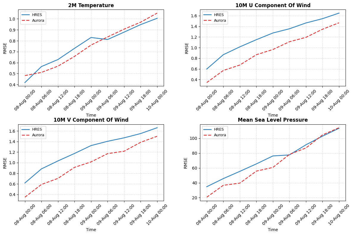
For 2-meter temperature, Aurora and HRES perform very similarly. HRES begins with slightly lower error immediately after initialization, but Aurora quickly catches up, and by 9 August the two curves are nearly indistinguishable. Both models show steadily increasing RMSE with forecast lead time, which is expected, but neither gains a clear advantage. This indicates that Aurora is essentially on par with HRES in predicting near-surface temperature.
For the 10-meter wind components, Aurora shows a consistent advantage. In both the U and V components, the Aurora RMSE remains systematically lower than HRES throughout the forecast period. The gap is fairly stable, suggesting that Aurora maintains better skill in capturing near-surface wind variability. This is a notable result, since wind fields are typically more difficult to predict than temperature or pressure, and Aurora appears to outperform the operational model here.
The situation is slightly different for mean sea level pressure. At very short lead times, HRES has a small advantage, reflecting its direct assimilation of observations into the initial conditions. However, Aurora steadily reduces the gap and by the second day the two models perform almost identically. Over the remainder of the forecast window, their errors evolve in parallel, showing essentially equivalent skill.
Taken together, these comparisons show that Aurora is at least competitive with HRES, and in some cases superior. For surface winds, Aurora provides consistently better forecasts, while for near-surface temperature and pressure the two models are broadly comparable.
The fact that Aurora can match or surpass HRES performance in multiple key variables highlights the strength of deep learning–based forecasting systems relative to traditional NWP.