DLESyM Output Analysis
Several weeks ago, a new climate AI model, DLESyM, was released. This model represents a major development in the use of deep learning for Earth system science, with an explicit focus on coupling the ocean and atmosphere.
In this post, I will provide an overview of the model’s architecture, and present some initial analysis of its output. The emphasis will be on two critical aspects: how well the model maintains long-term climate stability, and representation of extreme events. These are essential for assessing whether AI-based climate models can provide reliable simulations alongside traditional physics-based approaches.
The full code for this post can be found on GitHub.
DLESyM Architecture
DLESyM was trained primarily on ERA5 reanalysis data, with the addition of outgoing longwave radiation from the International Satellite Cloud Climatology Project (ISCCP).
A key feature of DLESyM is its use of a HEALPixgrid rather than a standard latitude–longitude grid. The HEALPix grid is divided into 12 faces, each with a 64×64 resolution.
This approach is advantageous for global climate modeling because, due to the curvature of the Earth, regions defined on a regular latitude–longitude grid can have unequal surface areas, particularly near the poles. The HEALPix grid provides nearly equal-area cells, improving the representation of spatial statistics and ensuring that global averages and distributions are not biased by variations in cell size.
It’ll imoprtant to keep this in mind at various points in the below analysis.
The model predicts a set of key atmospheric and oceanic variables, summarized in the table below:
| Model | Variable |
|---|---|
| atmos | outgoing longwave radiation (olr) |
| atmos | 2m temperature (t2m0) |
| atmos | 850-hPa temperature (t850) |
| atmos | 700–300-hPa geopotential difference (tau300-700) |
| atmos | total column water vapor (tcwv0) |
| atmos | 10-m horizontal windspeed magnitude (ws10) |
| atmos | 1000-hPa geopotential height (z1000) |
| atmos | 500-hPa geopotential height (z500) |
| atmos | 250-hPa geopotential height (z250) |
| ocean | surface sea temperature (sst) |
At its core, DLESyM employs two U-Net style convolutional neural networks in an autoregressive rollout framework: one for the atmosphere and one for the ocean. A separate module was developed for precipitation, but in this analysis, the focus is on the coupled atmosphere–ocean components.
The atmospheric network follows a three-level U-Net architecture, with channel depths of 180, 90, and 90, respectively. Two architectural components are central to its design:
- ConvNeXt blocks Liu et al., 2022 implemented with $1 \times 1$ kernels to reduce the number of trainable weights while enabling deeper latent layers.
- Convolutional Gated Recurrent Unit (GRU) layers Cho et al., 2015, which help capture temporal dependencies across successive steps.
The network is trained to minimise the global root mean squared error (RMSE) over 24 hours, using 6-hourly data generated by two consecutive steps. Optimising over a 24-hour horizon allows the model to learn full diurnal variability across the globe without biasing it toward multi-day ensemble mean states.
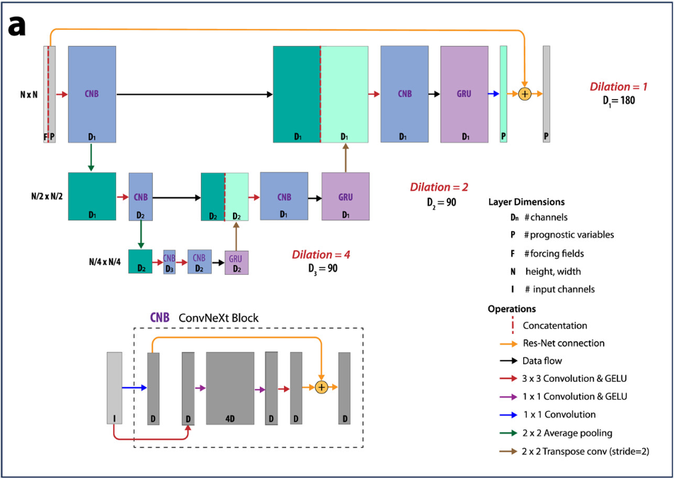
The oceanic module mirrors the U-Net design but is considerably smaller, with channel depths of 90, 45, and 45. Unlike the atmospheric model, the GRU layers were omitted, reflecting the relative simplicity of the system (the ocean module predicts only sea-surface temperature).
Because the ocean evolves on slower timescales than the atmosphere, the two modules operate with different update frequencies:
- Atmosphere: updated every 12 hours, producing 6-hr and 12-hr forecasts.
- Ocean: updated every 4 days, producing forecasts at 48-hr and 96-hr intervals.
The coupling proceeds in 96-hour cycles. The atmosphere is first advanced forward in 12-hour steps to generate forecasts up to 96 hours. These predictions are averaged and used to drive the ocean model over the same 96-hour window. Coupling in this context means that the two models exchange variables. At the coupling times, the atmosphere modle passes $WS_{10}$, $z_{1000}, and $OLR$ to the ocean model, while the ocean model passes $SST$ to the atmosphere model.
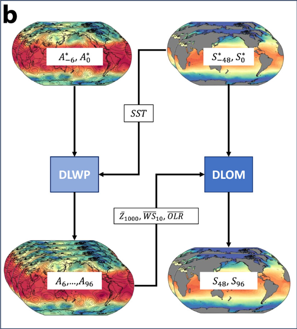
This iterative process maintains long-term stability of the coupled system. A key design choice is that near-surface air temperature is deliberately excluded from the coupling, to avoid artificial feedback loops. The rationale is that sea-surface temperature acts as a primary driver of the atmosphere, while the reverse influence is secondary and more prone to spurious correlations if imposed directly.
Output Analysis
The first thing to do was to generate the output.
Since the output is roughly 250GB, I opted for storing the it in a Google bucket. To do this, I forked the original repo and modified it so that the output data is saved to a zarr file. My fork can be found here. I also hired some GPUs to do the job, it took about an hour and a half for the 100 year simulation. The Google bucket is not publicly available, but if you’d like to access the dataset, pleast don’t hesitate to reach out.
Since DLESyM does not incoporate anthropenic forcing, the simulations express an equilibrium climate, implying that over the long term, we should expect to see the statistical properties (e.g. averages, distributions) of the output remain the same.
Climate Drift
The first step in analyzing the model’s climate output is to compute global, annual averages for each variable over the full simulation period. To quantify long-term stability, a linear regression line can then be fitted to these averages.
An ideal model exhibits a near-flat regression line. While natural variability is expected at shorter timescales, a pronounced slope—indicating a persistent warming or cooling trend—would reveal instability in the model.
With xarray, this procedure is straightforward. For each variable, yearly means are calculated to produce a time series of 100 points. A linear regression is then performed on this series.
# calc_annual_averages.py
import xarray as xr
from sklearn.linear_model import LinearRegression

def get_annual_averages(dataset: xr.Dataset) -> xr.Dataset:
    annual_averages = (
        dataset.resample(step='YE')
        .mean(dim=['step', 'face', 'height', 'width'])
        .isel(step=slice(None, -1))
    )
    return annual_averages.compute()

ocean_ds = xr.open_zarr(run_args.ocean_store)
atmos_ds = xr.open_zarr(run_args.atmos_store)

ocean_averages = get_annual_averages(ocean_ds)
atmos_averages = get_annual_averages(atmos_ds)

# Run regression and get drift
var_name = "sst"
data = ocean_averages[var_name]
lin = LinearRegression()
X = data.step.values.astype("datetime64[D]").astype(float).reshape(-1, 1)
y = data.values
lin.fit(X, y)
regression_line = lin.predict(X)
drift = lin.coef_[0]
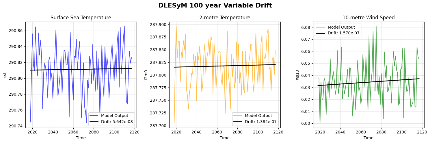
Across all three panels, the model exhibits substantial short-term variability, reflecting natural fluctuations in the coupled atmosphere–ocean system. However, the fitted linear trends confirm that the system remains stable over the long term. These results demonstrate that despite short-term noise, DLESyM maintains equilibrium in key atmospheric and oceanic variables without significant systematic drift.
Distribution Stability
Another perspective on model stability is to examine whether the distributions of variable values remain consistent over the simulation period.
In the analysis below, histograms are produced for the first decade (2017–2027) and the last decade (2107–2117) for sea-surface temperature, 2-meter air temperature, and wind speed. By directly comparing these histograms, we can assess whether the distributions have changed over time. For reference, ERA5 histograms from 2007–2017 are also included. Although not a strictly comparable period, these provide context for how DLESyM reproduces observed climatological distributions.
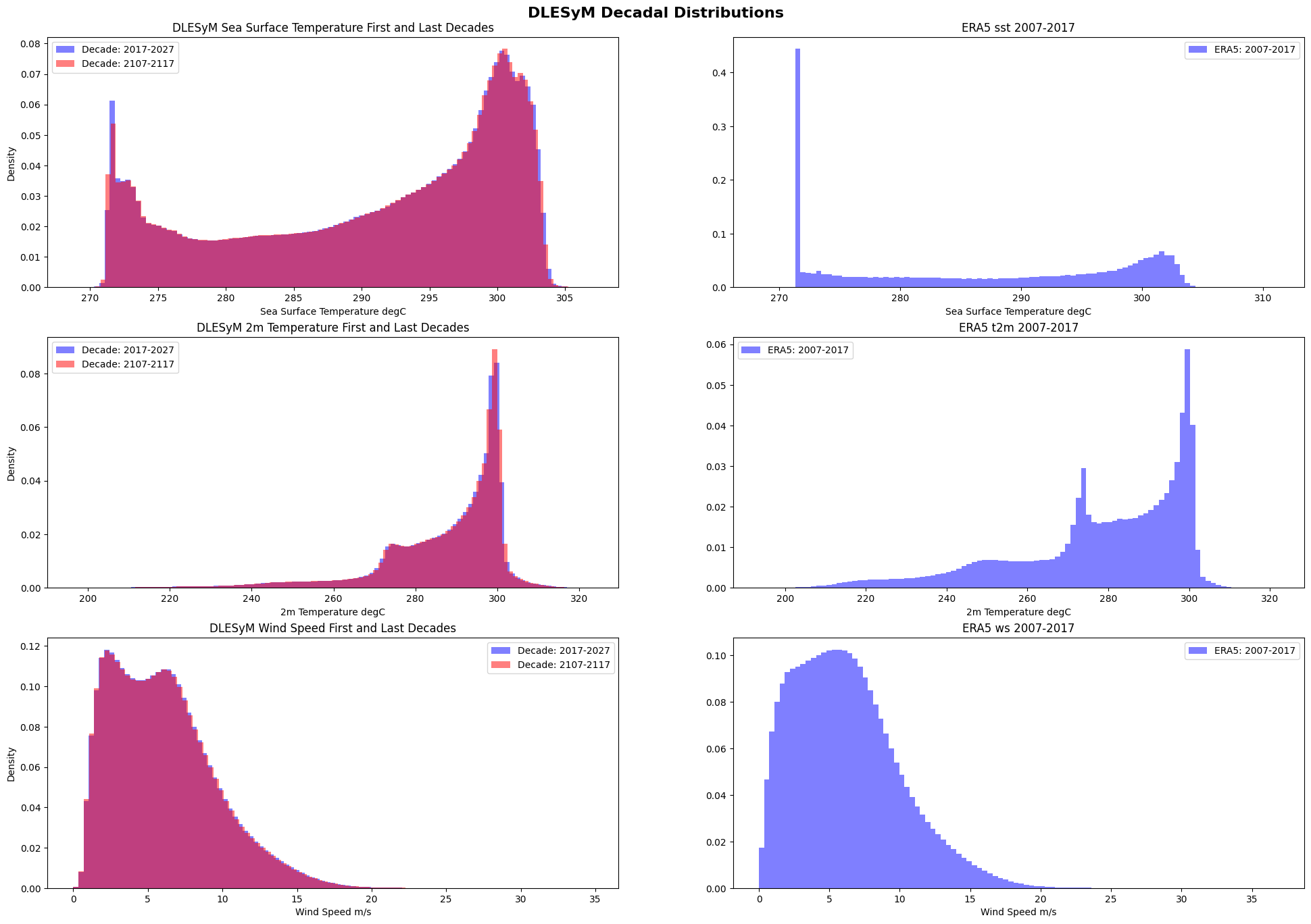
The left panels show DLESyM distributions for the first and last decades of the simulation, while the right panels show ERA5 reference distributions.
Sea-Surface Temperature: The DLESyM SST distribution exhibits characteristic bimodality, with a strong peak near the freezing point (~271 K) and a broader concentration between 295–305 K. Differences between the first and last decades are minimal. Compared to ERA5, the model produces a smoother SST distribution, with a less pronounced freezing-point peak and slightly narrower upper tails. ERA5 shows a sharper 271 K peak, reflecting the physical constraint of seawater freezing, which the model represents in a more diffuse manner.
2-Meter Air Temperature: Distributions for the first and last decades almost perfectly overlap. DLESyM produces a slightly narrower distribution than ERA5, with fewer extreme cold events and an upper tail more sharply centered near 300 K. ERA5 shows stronger multimodality, with distinct peaks corresponding to climatological regimes such as polar, midlatitude, and tropical zones. DLESyM smooths over these distinctions, capturing the mean state but underrepresenting the heterogeneity of climate zones.
Wind Speed: Distributions show the closest agreement with ERA5. Both exhibit a right-skewed pattern, with most values below 10 m/s and a long tail to higher speeds. Early and late DLESyM decades are nearly identical, and the overall distribution aligns closely with ERA5, indicating strong consistency in modeled wind statistics over time.
Percentiles
Another approach to evaluating the stability and realism of DLESyM outputs is to examine the temporal evolution of extreme values through percentiles.
We calculate the 75th, 90th, 95th, and 99th percentiles for each variable at each grid point on each day of the year across the entire 100-year simulation. This provides insight into both moderate and extreme conditions, highlighting how well the model represents variability and rare events over long timescales.
Again, by using xarray, this procedure is straightforward. The function below efficiently computes these percentiles across the HealPix grid for all time steps:
import xarray as xr

PERCENTILES = [0.75, 0.90, 0.95, 0.99]

def get_quantiles(dataset: xr.Dataset) -> xr.Dataset:
    quantiles = dataset.groupby("step.dayofyear").quantile(PERCENTILES)
    return quantiles
From the computed percentiles, we can visualize the temporal and spatial structure of extremes. In the analysis below, we focus on sea-surface temperature.
First, we examine the seasonal cycle of selected percentiles at a specific Northern Hemisphere location.
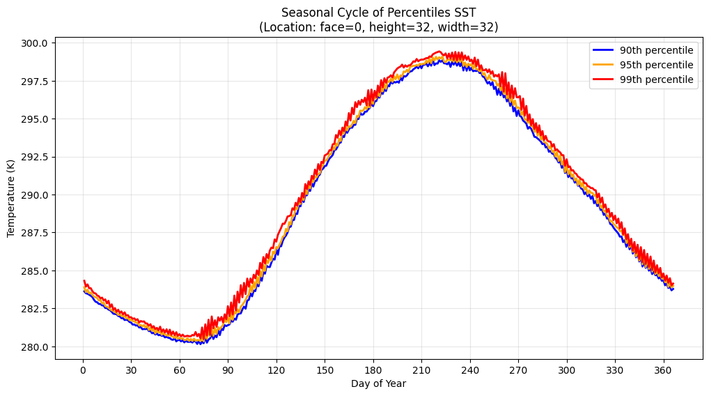
All three percentiles follow a pronounced annual cycle, with minimum temperatures in winter (around days 50–80) and maximum temperatures in summer (around days 200–250). This indicates strong seasonality in SST at this location.
However, note the tight spread between the percentiles. The difference between the 90th and 99th percentiles is small, on the order of 1–2 K. This suggests that even extreme values remain relatively close to the upper quantiles of the distribution, pointing to limited variability in the upper tail.
The higher percentiles (particularly the 99th) display higher-frequency fluctuations superimposed on the seasonal cycle. This could reflect short-lived warming events, likely tied to transient atmospheric forcing or mesoscale ocean variability
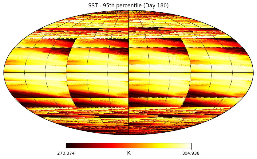
In the above figure, we consider the percentiles of SST at all spatial points on Day 180, corresponding to late June, or midsummer in the Northern Hemisphere. The visualisation uses a Mollweide projection, a standard approach for global data on a HealPix grid.
The color scale ranges from approximately 270.4 K to 304.9 K (about -2.75°C to 30.85°C), with cooler temperatures rendered in dark reds and blacks, and the warmest regions shown in yellow and white.
A pronounced latitudinal pattern is evident, consistent with the global climate zones that shape SST distributions. Equatorial oceans exhibit the highest SSTs, particularly in tropical regions where solar insolation is strongest and seasonal variability is minimal
This spatial view confirms that DLESyM captures the large-scale climatological gradients of SST while preserving expected latitudinal patterns, providing confidence in the model’s representation of global oceanic structure.